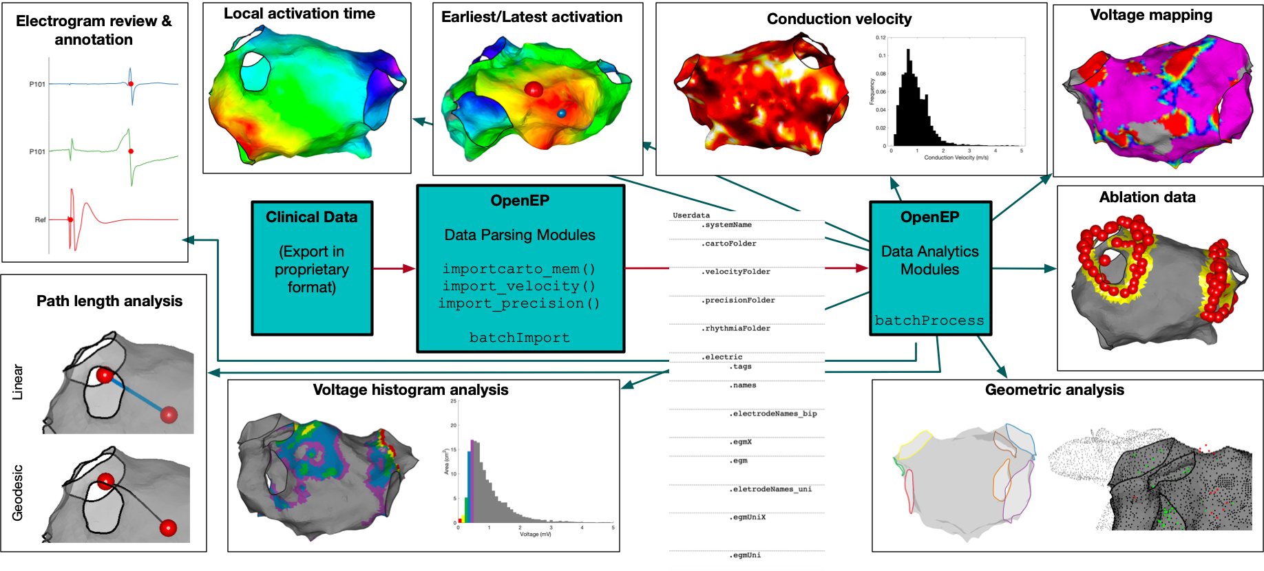
 The figure above shows the key components of the OpenEP framework. There is a Data Parsing module which is used to convert proprietary electroanatomic mapping formats into the OpenEP data format. There are the Data Analytics modules which are used to visualise, interpret and analyse OpenEP data. Since these modules make use of the OpenEP data format, once electroanatomic mapping data is in this format each of these modules can be used to process the data. OpenEP data analysis modules are available to process activation data, voltage data, ablation data and geometric data.
This page details some examples on how to use the OpenEP framework. Please click through the links below. All the example data necessary for running the examples is given in the source code repository.
Please contact us if you have a particular analysis technique that you would like to perform but haven't yet implemented - the OpenEP framework will almost certainly simplify your work!
The figure above shows the key components of the OpenEP framework. There is a Data Parsing module which is used to convert proprietary electroanatomic mapping formats into the OpenEP data format. There are the Data Analytics modules which are used to visualise, interpret and analyse OpenEP data. Since these modules make use of the OpenEP data format, once electroanatomic mapping data is in this format each of these modules can be used to process the data. OpenEP data analysis modules are available to process activation data, voltage data, ablation data and geometric data.
This page details some examples on how to use the OpenEP framework. Please click through the links below. All the example data necessary for running the examples is given in the source code repository.
Please contact us if you have a particular analysis technique that you would like to perform but haven't yet implemented - the OpenEP framework will almost certainly simplify your work!
Ablation quantification
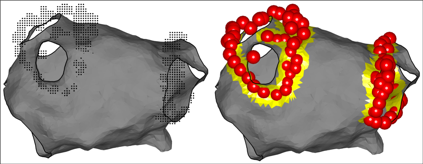 OpenEP can be used to display representations of ablation points and to quantify the ablation area. The worked-through example here uses “visitag” data from the Carto3 electroanatomic mapping platform. This data is not loaded automatically using a call to importcarto_mem and needs to be loaded separately. This is done by using the following code, but has already been done for Example 1.
folderPath = <path to the visitag folder>
userdata = importvisitag(userdata, folderPath)
To run this example, load Example 1:
load openep_dataset_1.mat;
To display ablation lesions:
% Display using defaults
plotVisitags(userdata, 'orientation', 'ap');

% Change the ablation lesion colour
plotVisitags(userdata, 'orientation', 'ap', 'colour', 'b');

% Colour ablation lesions according to the rf index value (in this case the Ablation Index)
plotVisitags(userdata, 'orientation', 'ap', 'colour', userdata.rfindex.tag.index.value);

% Show only the ablation lesions and not the shell
plotVisitags(userdata, 'orientation', 'ap', 'colour', userdata.rfindex.tag.index.value, 'shell', 'off');
For visitag data, the co-ordinates of the grid can also be accessed and displayed.
% With the shell
plotVisitags(userdata, 'plot', 'grid')

% Without the shell
plotVisitags(userdata, 'plot', 'grid', 'shell', 'off')
To calculate the area of tissue ablated, use the getAblationArea.m function.
% Calculate the total ablation area
ablArea = getAblationArea(userdata)

% Access the ablation area as a triangulation
[~, ~, trAbl] = getAblationArea( userdata )

% Plot the ablation area
plotAblationArea(userdata)
API Links
getAblationArea.m plotAblationArea.m plotVisitags.m importvisitag.m
Activation mapping
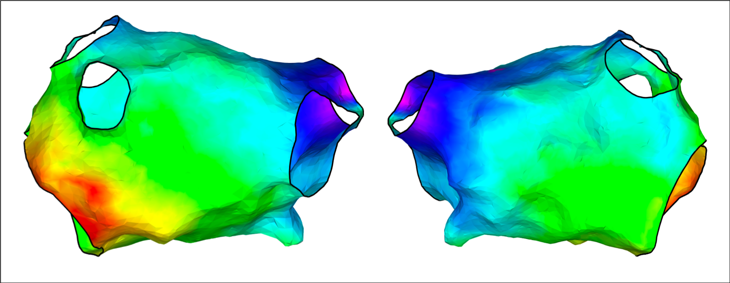
Local activation time maps created by the clinical mapping system can be displayed using the OpenEP framework. Local activation time maps can also be re-interpolated from raw electrogram data by OpenEP (see generateInterpData.m) and the resulting interpolated maps displayed using OpenEP.
To run this example, load Example 1:
load openep_dataset_1.mat;
Display the activation map created by the clinical electroanatomic mapping system:
% Since the data already exists, we can call drawMap.m directly, specifying 'type' = 'act'
drawMap(userdata, 'type', 'act');

% Change the orientation of the map using the 'orientation' flag
drawMap(userdata, 'type', 'act', 'orientation', 'ap'); % antero-posterior orientation
drawMap(userdata, 'type', 'act', 'orientation', 'pa'); % postero-anterior orientation

% Change the window of interest to cover the earliest 10% of electrograms
activationTimes = getSurfaceData(userdata, 'act');
tMin = nanmin(activationTimes);
tMax = nanmax(activationTimes);
tRange = tMax - tMin;
tEnd = tMin + floor(tRange*0.1);
drawMap(userdata, 'type', 'act', 'orientation', 'pa', 'coloraxis', [tMin tEnd]);
Re-interpolate an activation map from the raw electrogram data and subsequently display an activation map:
interpData = generateInterpData(userdata, 'lat-map');
drawMap(userdata, 'type', 'act', 'orientation', 'ap', 'data', interpData);
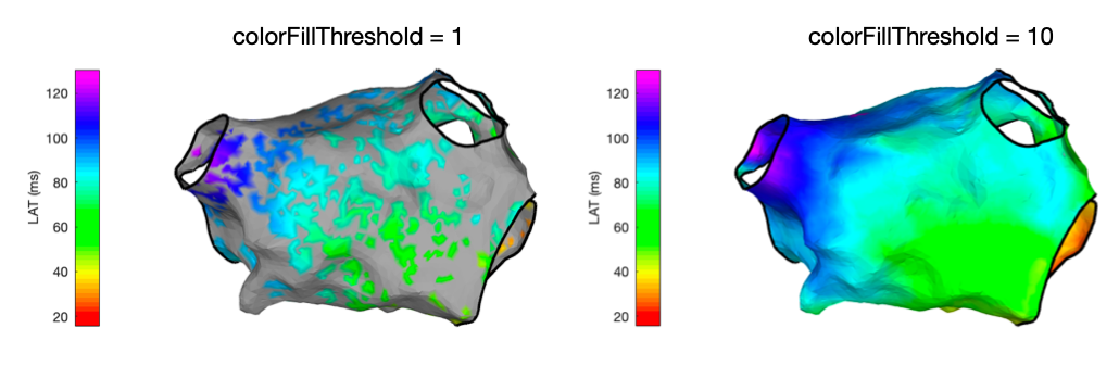
Change the fill threshold (default = 10)
% Use default value of colorFillThreshold
colorFillThreshold = 10;
drawMap(userdata, 'type', 'act', 'orientation', 'ap', 'data', interpData, 'colorfillthreshold', colorFillThreshold);

% Change colorFillThreshold to 1
colorFillThreshold = 1;
drawMap(userdata, 'type', 'act', 'orientation', 'ap', 'data', interpData, 'colorfillthreshold', colorFillThreshold);
API Links
drawMap.m getSurfaceData.m generateInterpData.m
Conduction velocity
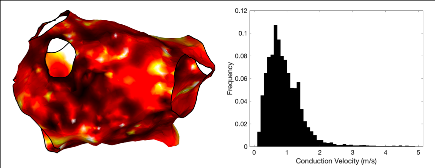
OpenEP includes functions to create conduction velocity maps from local activation time maps, which can be displayed using the drawMap.m function. In addition, conduction velocity histogram analysis is available via the cvHistogram.m function. A triangulation-based method to calculate the gradient of local activation times is employed to calculate conduction velocities independent of wavefront direction.
To run this example, load Example 1:
load openep_dataset_1.mat;
There are now two options. Firstly, drawMap.m can be used directly to calculate the conduction velocity data and draw the figure.
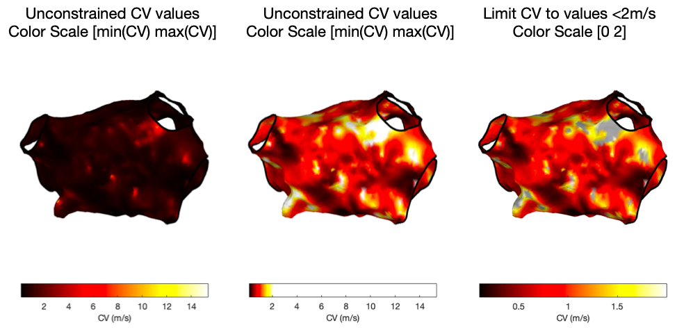
% Automatic colour scale
drawMap(userdata, 'type', 'cv', 'orientation', 'ap');

% Limit colour scale to physiological values
drawMap(userdata, 'type', 'cv', 'orientation', 'ap', 'coloraxis', [0 2]);
Alternatively, the 'data' flag of the drawMap.m function can be used, together with getConductionVelocity.m which will return the conduction velocity data. This method can be used, for example, to remove non-physiological values before plotting.
cvdata = getConductionVelocity(userdata);
cvdata(cvdata>2) = NaN;
drawMap(userdata, 'type', 'cv', 'orientation', 'ap', 'data', cvdata);
Examples of all three maps are shown below.
OpenEP can also draw histograms of the conduction velocity.
% default settings
cvHistogram(userdata);

% show all the data
cvHistogram(userdata, 'limits', [-Inf Inf]);

% limit to physiological values
cvHistogram(userdata, 'limits', [0 2]);

% adjust the bin width
cvHistogram(userdata, 'limits', [0 2], 'binwidth', 0.01);
API Links
getConductionVelocity.m drawMap.m cvHistogram.m
Data input, storage and batch processing
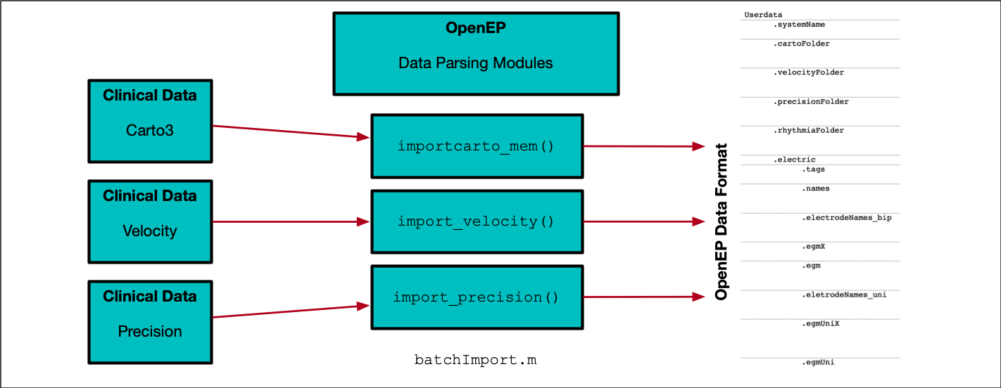
The Data Parsing modules serve to convert proprietary electroanatomic mapping export dataformats into the OpenEP data format. There are several ways to use the import functions including in semi-graphical mode and command line mode.
% Semi graphical mode
userdata = importcarto_mem()

% Command line mode
studyXmlFile = <path to study XML file> (string)
maptoread = <name of map> (string)
refchannel = 'CS9-CS10';
ecgchannel = 'V1';
savefilename = '~/openep/data/1.mat'
userdata = importcarto_mem(studyXmlFile, 'maptoread', maptoread, 'refchannel', refchannel, 'ecgchannel', ecgchannel, 'savefilename', savefilename)
In command line mode, the map to read can also be identified by the number of points in that map, as long as the number of points in the map of interest is unique for that case. For example, for a map containing 1059 points:
studyXmlFile = <path to study XML file> (string)
maptoread = 1059
refchannel = 'CS9-CS10';
ecgchannel = 'V1';
savefilename = '~/openep/data/1.mat'
userdata = importcarto_mem(studyXmlFile, 'maptoread', maptoread, 'refchannel', refchannel, 'ecgchannel', ecgchannel, 'savefilename', savefilename)
Fully automating import, for example of a set of study files is a more complicated process which requires copy the data from its original location, unzipping the data, identifying the study XML file, identifying the map and performing the input. It is recommended to use batchImport.m, modified where necessary, to perform these tasks.
batchImport
To process multiple OpenEP datasets, an example batch processing script is also provided and can be modified to use any of the OpenEP data analysis modules.
batchProcess
API Links
importcarto_mem.m batchImport.m
Earliest/Latest activation
OpenEP provides modules for calculating the site of earliest activation and the site of latest activation on a local activation time map. These positions can be used, for example, to measure the chamber total activation or identify the earliest activation site closest to a pacing site. A number of different methods are provided for identifying these sites as outlined below.
To run these examples, load Example 1:
load openep_dataset_1.mat;
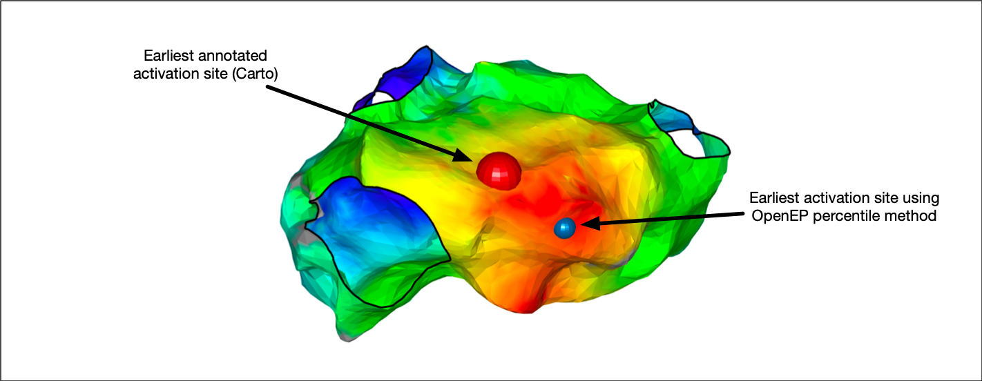
First, we can access the site of earliest activation consistent with the clinical mapping system. This is defined as the earliest point on the interpolated activation map and is accessed as follows:
X = getEarliestActivationSite(userdata, 'method', 'clinmap');
This OpenEP function call returns the Cartesian co-ordinates of the earliest activating point on the local activation time map.
We can also return the index of the mapping point closest to this activating site, along with the activation time, relative to the reference annotation.
[X, ~, iPoint, t] = getEarliestActivationSite(userdata, 'method', 'clinmap');
If we are only interested in the earliest activation times recorded on an actual electrogram, rather than interpolated on the activation map, then we can access that, too:
[X, surfX, iPoint, t] = getEarliestActivationSite(userdata, 'method', 'ptbased');
Here, we have returned two Cartesian co-ordinates, X and surfX. Using getEarliestActivationSite.m (or getLatestActivationSite.m) with the 'method' flag set to 'ptbased' returns the Cartesian co-ordinates of the earliest annotated electrogram (X) as well as its surface projection (surfX).
Basing the site of earliest/latest activation on the very earliest map point or electrogram point can be error-prone if for example, there is a single point which is annotated too early. OpenEP therefore provides percentile methods where the earliest 2.5th percentile (or latest 2.5th percentile) electrograms or surface mapping points are first identified, then the mean of their x, y and z co-ordinates are calculated. These methods are accessed by setting the 'method' flag to 'ptbasedprct' or 'clinmapprct'. For example:
% electrogram based calculation
[X, surfX, iPoint, t] = getEarliestActivationSite(userdata, 'method', 'ptbasedprct');

% map based calculation
[X, surfX, iPoint, t] = getEarliestActivationSite(userdata, 'method', 'clinmapprct');
Three final observations:
- Rather than using the interpolated map created by the clinical mapping system, we can also re-interpolate the activation map using OpenEP. This is desirable if, for example, data is being analysed from multiple mapping systems for a single study. The equivalent methods are
'openepmap'and'openepmapprct'. - The percentile used for the percentile-based methods can be changed from the default of 2.5 by using the
'prct'flag and passing in a double value. - Whilst the above discussion has focussed on
getEarliestActivationSite.mthe same parameter/value pairs are used to customise the functiongetLatestActivationSite.m.
API Links
getEarliestActivationSite.m getLatestActivationSite.m
Electrogram display/annotation
Although electroanatomic mapping systems provide detailed mapping representations of eletrophysiological data sometimes it is essential to access the individual electrograms which are used to create these maps. For example, it might be desirable to provide desirable to apply a uniform interpolation scheme across data collected by different mapping systems. Or, the purpose of a study may be to analyse electrogram characteristics in ways which are not currently implemented in the clinical systems. OpenEP therefore provides methods to access and display electrogram data for such purposes.
To run this example, load Example 1 or Example 2:
load openep_dataset_1.mat;
% or
load openep_dataset_2.mat;
In order to identify the electrogram of interest it is necessary to know the point number of that point which can be identified from the 'userdata' or from the clinical system. Note that in the case of Carto data it is necessary to convert the point number displayed on the clinical system into the point number used within OpenEP:
pointNumber = 1042; % for example
iEgm = getIndexFromCartoPointNumber(userdata,pointNumber))
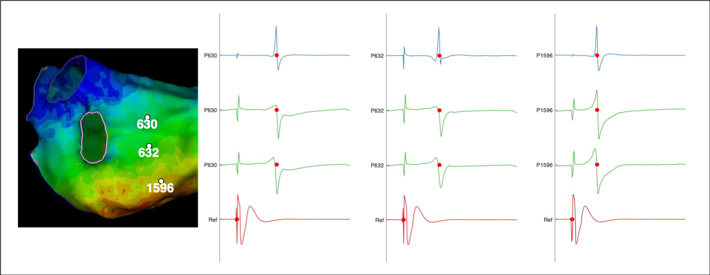
Once we have the correct index for the desired point number we can plot the electrograms associated with that point using plotOpenEPEgms.m
plotOpenEPEgms(userdata, 'iegm', iEgm)
A call to plotOpenEPEgms.m such as the above will, by default, plot the bipolar electrogram associated with the mapping point together with the associated unipolar mapping pair. The range of the plotted electrogram will be equivalent to the mapping window with a buffer of 50 samples before and after applied. The reference and electrogram channels will both be shown on the plot. All of these preferences can be changed using the appropriate parameter/value pairs (see the API documentation for the full list). For example, if we do not want to show the reference channel we can call the following:
plotOpenEPEgms(userdata, 'iegm', iEgm, 'reference', 'off')
Similarly, if we only want to show the bipolar electrogram then we can call the following:
plotOpenEPEgms(userdata, 'iegm', iEgm, 'egmtype', 'bip')
For signal processing purposes it is necessary not just to display the electrograms but to access the raw electrogram data. This is done via the OpenEP function getEgmsAtPoints.m. For example, if we want to access the bipolar electrogram associated with the above mapping point then we would call:
egmTraces = getEgmsAtPoints(userdata, 'iegm', iEgm, 'egmtype', 'bip');
If we also wanted the unipolar electrograms then we would call the following (or simply not specify 'egmtype'):
egmTraces = getEgmsAtPoints(userdata, 'iegm', iEgm, 'egmtype', 'bip-uni');
In addition to returning the raw electrograms, the OpenEP function 'getEgmsAtPoints.m' can also be used to access the annotations and the electrogram names, which are returned as additional output arguments:
[egmTraces, acttime, egmNames ] = getEgmsAtPoints(userdata, 'iegm', iEgm);
When working with the electrogram data, it can be useful to access the windows of interest. A getter function is planned in the OpenEP Roadmap to expose this information. For now it can be accessed at the low level by directly interrogating userdata and is stored in the following location:
userdata.electric.annotations.woi
One final observation:
- A key step in creating maps in OpenEP is to identify the mapping points which have annotations within the window of interest. Note that OpenEP does not currently provide functionalities for editing the annotations. Instead, any electrograms with annotations outwith the window of interest could be identified and discarded in your algorithms before processing. The OpenEP function
'getMappingPointsWithinWoI.m'is provided for this purpose:iPoint = getMappingPointsWithinWoI(userdata);
API Links
getIndexFromCartoPointNumber.m plotOpenEPEgms.m getEgmsAtPoints.m getMappingPointsWithinWoI.m
Geometry analysis
 OpenEP provides some tools for analysing the geometry stored in OpenEP data format. These tools are particularly important for electroanatomic mapping data analysis since they are quantifiable and avoid any ambiguity regarding how similar metrics are calculated in clinical systems. Their use has been validated and OpenEP users are strongly encouraged to use these methods rather than the equivalent methods available in the clinical electroanatomic mapping systems.
To run this example, load a dataset:
load openep_dataset_1.mat;
Chamber shape and size
OpenEP can be used to calculate the area and the volume of the geometry stored in 'userdata'. For example, to calculate the area, simply call:
area = getArea(userdata)
Similarly, to calculate the volume of the mapped chamber, simply call:
volume = getVolume(userdata)
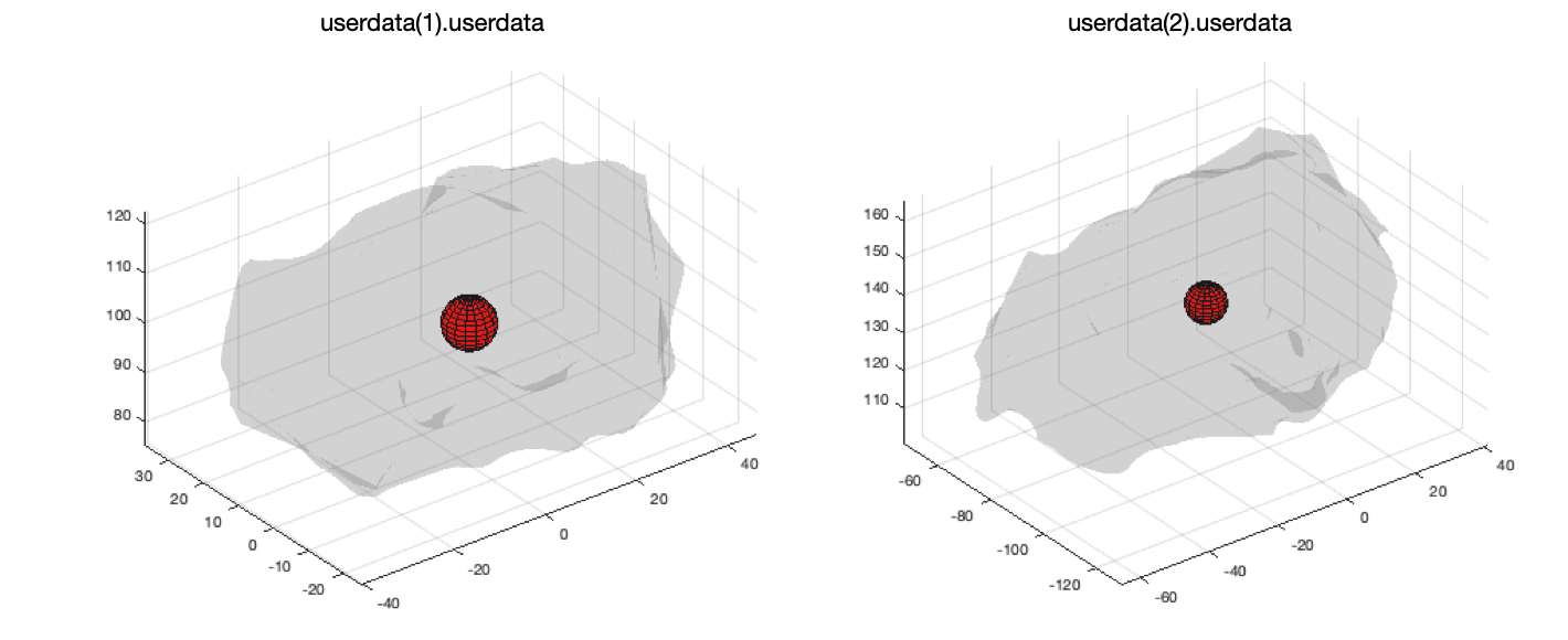
Another function that is particularly useful for standardising co-ordinate systems (for example for machine learning tasks) is to be able to centre all chambers around the same point. This can be done using 'getCentreOfMass.m' as follows:
% get two userdata objects
userdata(1) = load('openep_dataset_1.mat');
userdata(2) = load('openep_dataset_2.mat');

% calculate the centre of mass of each chamber and draw a figure
for i = 1:numel(userdata)
  figure
  C = getCentreOfMass(userdata(i).userdata, 'plot', true);
end
Once we have the co-ordinates of the centre of the mass they can be subtracted from the co-ordinates of the surface points to position the centre on the origin.
Structures and surfaces
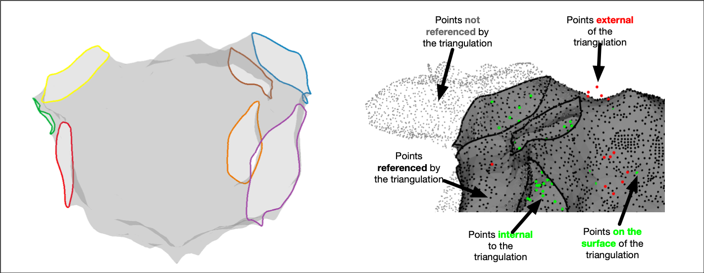
Anatomical structures are added to electroanatomic mapping system meshes in the form of orifices representing for example pulmonary vein ostia or valves. These anatomical structures are frequently used as important fiducial points for registration problems. OpenEP provides a function, getAnatomicalStructures.m to access these structures. For example:
% First, lets re-load the first example
load openep_dataset_1;

% Return the anatomical structures, but don't plot anything
FF = getAnatomicalStructures(userdata);

% Return the anatomical structures, and also plot a figure showing what was done
FF = getAnatomicalStructures(userdata, 'plot', true)
Calling the second of these function calls displays a figure representing the anatomical structures.
It is also possible to use getAnatomicalStructures.m to return information about each anatomical structure such as the perimeter and the area:
[~, l, a] = getAnatomicalStructures(userdata);
The same function, getAnatomicalStructures.m can create new triangulation representations of each anatomical structure:
[~, ~, ~, tr] = getAnatomicalStructures(userdata);
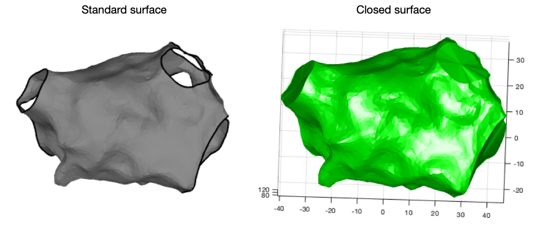
Sometimes it is desirable to create a closed surface where all the anatomical structures are ‘filled in’. OpenEP makes this process simple by providing the getClosedSurface.m function. Use this function as follows:
% call getClosedSurface.m
tr = getClosedSurface(userdata)

% create a figure of the results
drawMap(userdata, 'type', 'none')
figure
trisurf(tr, 'facecolor', 'g', 'edgecolor', 'none')
axis equal vis3d
cameraLight
Distances
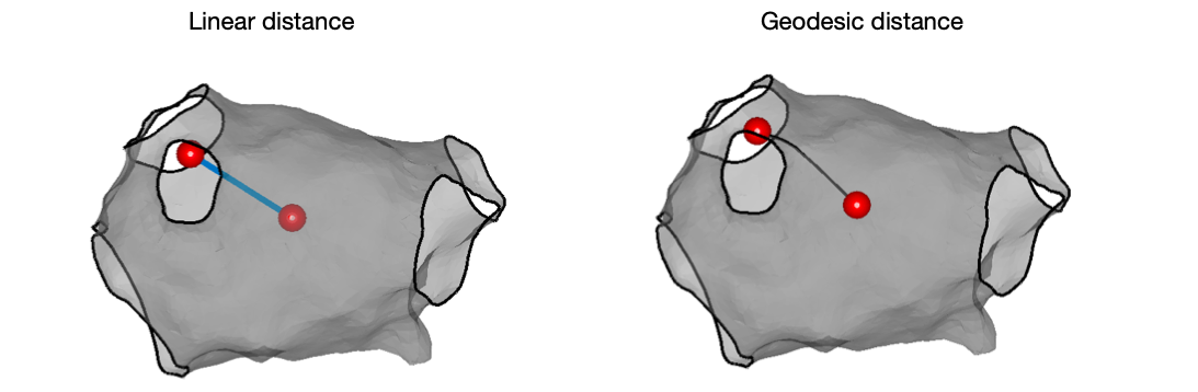
Calculating distances between mapping points, or between points on the surface of the mesh, is commonly performed for example to determine the size of a chamber, to determine the distance between ablation points, or to get a distance for use in a conduction velocity calculation. OpenEP provides two methods to calculate these distances. Distances can be calculated as a ‘straight line’ between two points. Such straight line distances will always be shorter than the distance across the surface of the shell. OpenEP also calculates therefore the geodesic distance across the surface of the shell. Use of the geodesic distance may make conduction velocity calculations more accurate, although this assertion will depend of course on the quality of the shell. To calculate such distances use distanceBetweenPoints.m. For example:
% linear method
distance = distanceBetweenPoints(userdata, 1, 100, 'plot', 'true', 'method', 'linear')

% geodesic method
distance = distanceBetweenPoints(userdata, 1, 100, 'plot', 'true', 'method', 'geodesic')
Mesh data
OpenEP provides the basic getter methods for accessing information about the mesh: getMesh.m, getVertices.m, getFaces.m:
mesh = getMesh(userdata);
vertices = getVertices(userdata);
faces = getFaces(userdata);
API Links
getArea.m getVolume.m getCentreOfMass.m getAnatomicalStructures.m getClosedSurface.m distanceBetweenPoints.m getFaces.m getMesh.m getVertices.m
Voltage mapping
 OpenEP provides a number of functions for displaying and analysing voltage maps. OpenEP can reproduce the voltage map created by the clinical electroanatomic mapping system. OpenEP can also create voltage maps de novo based on the electrogram data and a specified interpolation scheme. OpenEP can also perform analysis of low voltage areas, volage distributions and perform analysis of voltages falling within particular pre-set voltage ranges (voltage histogram analysis).
Conventional voltage mapping
To run these examples, load an example dataset:
load openep_dataset_1.mat;
First, lets draw a voltage map using the OpenEP function drawMap.m:
drawMap(userdata, 'type', 'bip', 'orientation', 'pa');
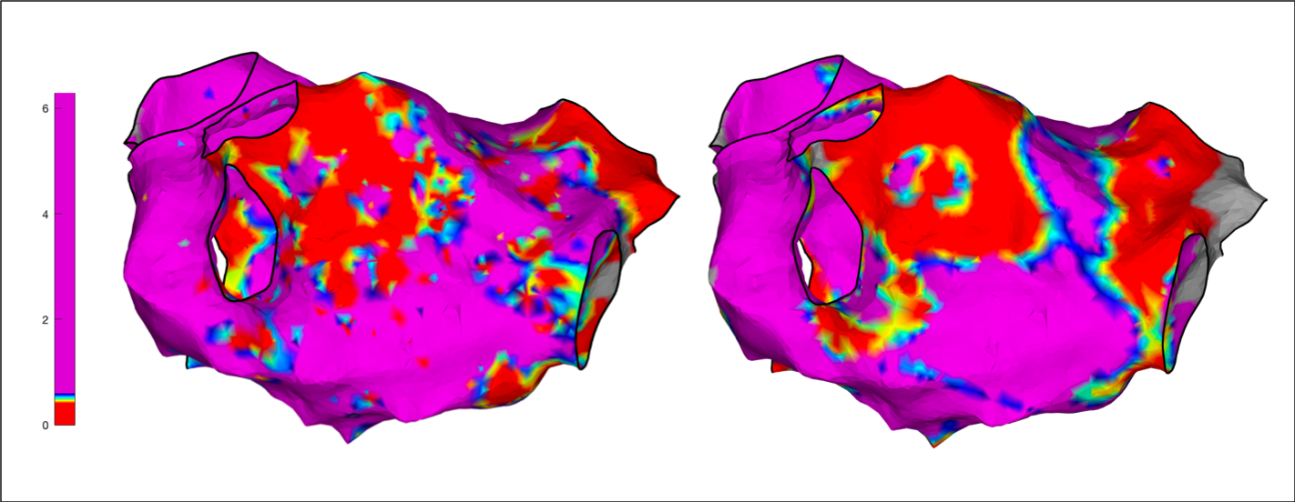
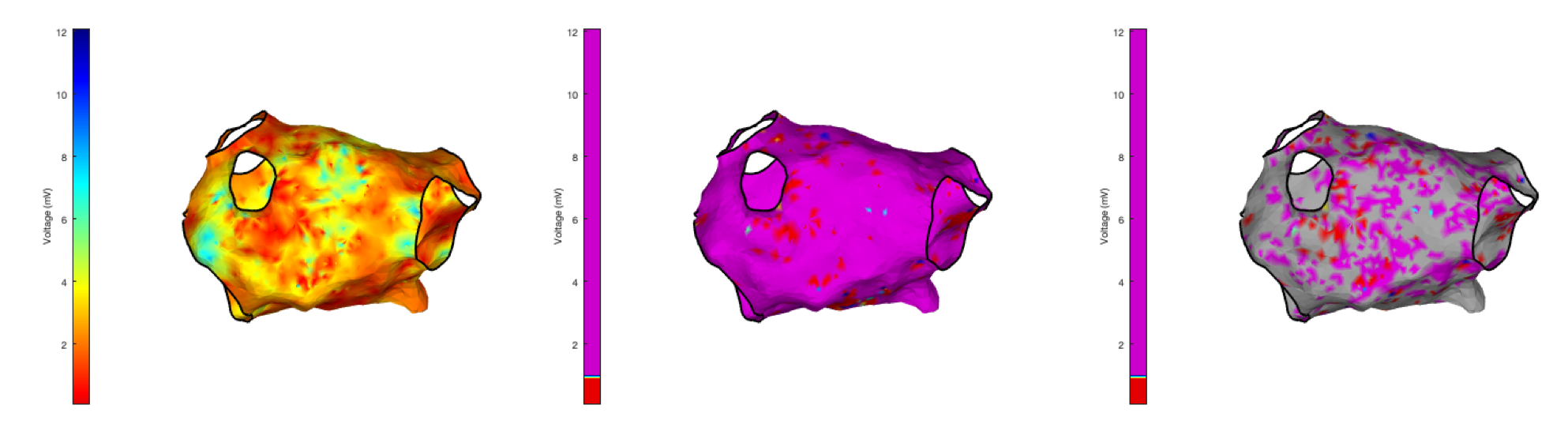
We can also specify the color window that we are interested in, for example to highlight low voltage areas; here specified as 1mV for effect.
drawMap(userdata, 'type', 'bip', 'orientation', 'pa', 'coloraxis', [0.9 1]);
We can also specify that we only want the map to be shaded within a certain distance of an actual mapping point; here shown as 1mm for effect.
drawMap(userdata, 'type', 'bip', 'orientation', 'pa', 'coloraxis', [0.9 1], 'colorfillthreshold', 1);
These three function calls should result in the figures shown below:
A common measurement made in contemporary electroanatomic mapping studies is to measure the area of a shell (both as an area and as a percentage) within which low voltage electrograms are recorded. OpenEP makes performing these calculations, and displaying the results, easy. The relevant function is getLowVoltageArea.m which is fully documented in the API reference. Some interesting features of this function are that it can calculate the low voltage area based on the mapping data exported by the electroanatomic mapping system, or by using the raw eletrograms. This latter method may be preferrably if a study is being performed which uses multiple different mapping platforms. If re-interpolation is required from raw electrogram data than getLowVoltageArea.m uses generateInterpData.m to reinterpolate a volage map first before calculating the required low voltage areas.
% Calculate area on the clinical electroanatomic map which has a bipolar voltage less than 0.5mV (default operation)
lowVArea = getLowVoltageArea(userdata)

% Change the low voltage threshold
lowVThreshold = [0 2];
lowVArea = getLowVoltageArea(userdata, 'threshold', lowVThreshold)
The first of these function calls returns a low voltage area of only 0.7cm^2, consistent with the figures above. By setting the low voltage area threshold to <2mV, a much larger area of 39.3cm^2 is returned as expected.
In order to present the low voltage areas as percentages of the total surface area you can make use of the OpenEP function getArea() as follows:
totalArea = getArea(userdata);
lowVPercentage = lowVArea/totalArea*100;
disp(['The low voltage area is ' num2str(lowVArea) 'cm^2 which is ' num2str(lowVPercentage) '% of the total area.'])
If you have been following along with this example then the output should be:
The low voltage area is 39.2615cm^2 which is 35.3819% of the total area.
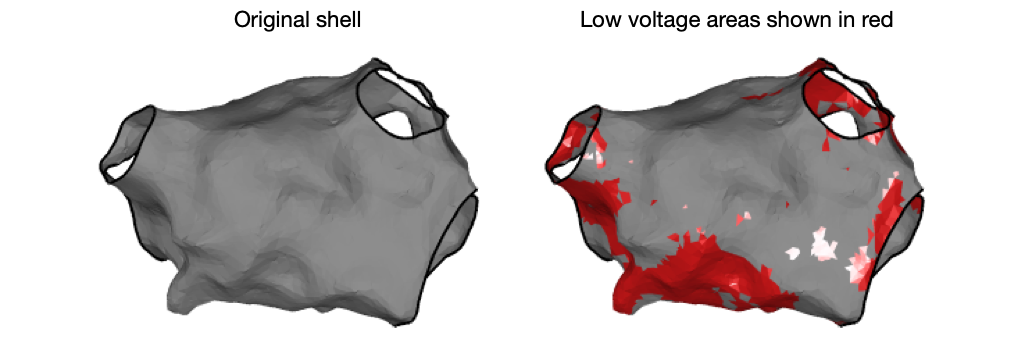
Helpfully, getLowVoltageArea.m also returns triangle indices as well as triangulation representations of the low voltage area. These can be used for visualisation of the low voltage area, for example:
[~, ~, ~, tr2] = getLowVoltageArea(userdata, 'threshold', lowVThreshold)
drawMap(userdata, 'type', 'none')
hold on
hS = trisurf(tr2, 'facecolor', colorBrewer('r'), 'edgecolor', 'none')
You can also calculate the mean voltage of an entire chamber using the OpenEP function getMeanVoltage.m. This function will calculate the mean voltage using either the map or the individual electrograms and can return both the mean bipolar voltage and the mean unipolar voltage, as shown below:
% calculate the mean bipolar voltage calculated from the mapping data
v = getMeanVoltage(userdata)

% calculate the mean bipolar voltage calculated from the raw electrograms
v = getMeanVoltage(userdata, 'method', 'egm')

% calculate the mean unipolar voltage
v = getMeanVoltage(userdata, 'method', 'egm', 'type', 'uni')
API Links
drawMap.m getLowVoltageArea.m getMeanVoltage.m generateInterpData.m
Voltage histogram analysis
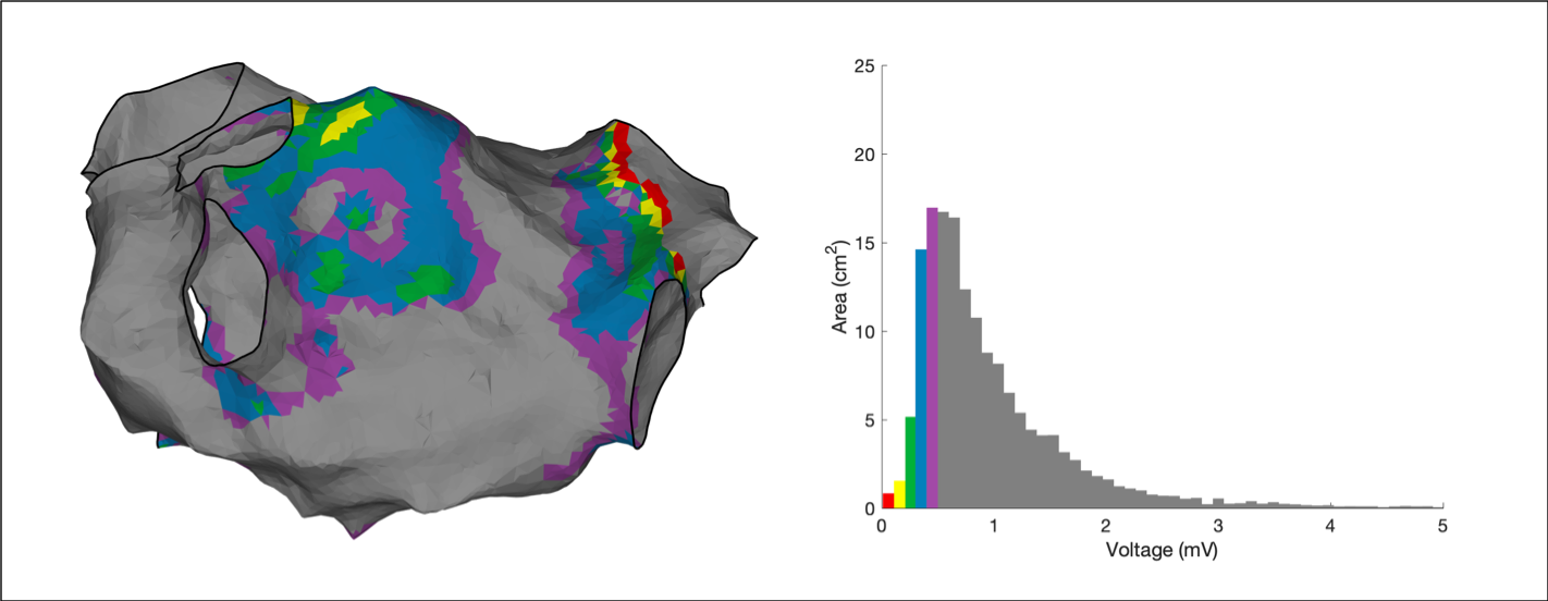 Voltage Histogram Analysis is an emerging technique which seeks to provide quantitative analysis of voltage maps over and above a low voltage area. Essentially, voltage histogram analysis is an extension of voltage area calculations where multiple areas are calculated each with a separate voltage range of interest. Voltage histogram analysis is provided through the OpenEP function
 voltageHistogramAnalysis.m. By default the ranges used are as previously published:
- 0.01 - 0.11mV
- 0.11 - 0.21mV
- 0.21 - 0.30mV
- 0.30 - 0.40mV
- 0.40 - 0.50mV
To perform voltage histogram analysis:
areas = voltageHistogramAnalysis(userdata)
Compared to the technique available in clinical systems, voltage histogram analysis performed in OpenEP can make use of the map-based data or the electrogram-based data, by setting 'method' to either 'map' or 'egm' and can operate on either unipolar or bipolar voltage data. See the API docs for full details.